Inserting pie chart in excel
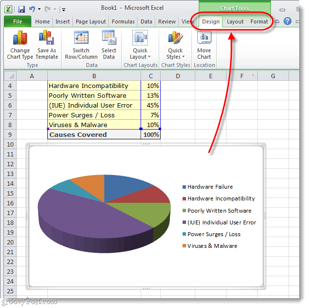
Inserting a new chart 42 Adding and removing labels 43 Entering chart data 44 Styling the chart 41 Inserting a new chart. We will click on the Design Tab.
How To Make A Pie Chart In Microsoft Excel 2010 Or 2007
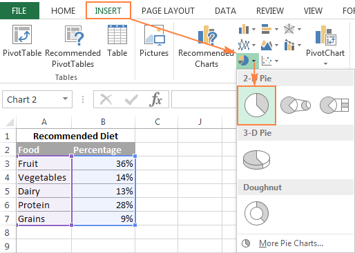
Inserting a Pie Chart.
. The article provides free Excel chart resources. In that case when you copy the chart keep it linked to the original Excel file. Select the cells in the rectangle A23 to B27.
Thats how to do a trendline in Excel. The address or name of a cell or a range of cells is known as Cell referenceIt helps the software to identify the cell from where the datavalue is to be used in the formula. The problem is that Excel doesnt have a built-in waterfall chart template.
A line chart in Excel is created to display trend graphs from time to time. Microsoft Excel 2019 Data Analysis and Business Modeling Sixth Edition. We will be inserting a graph on cells B1E2.
To change the value select cell D5 and rewrite the value to 10. To create a simple chart from scratch in Word click Insert Chart and pick the chart you want. Microsoft Excel 2010 Step by Step.
Keeping track of date and time helps in managing records of our work as well as segregate the information day-wise. Excel offers a variety of chart types based on your requirements. FormulaInfozip 36kb 26-Sep-12.
If you dont pass that argument by default the chart tries to plot by column and youll get a month-by-month comparison of sales. Microsoft Excel Basics Test. Study with Quizlet and memorize flashcards containing terms like To change the name of a worksheet you rename the _____.
We can customize the graph after inserting. Download Free PDF View PDF. Comparison Chart in Excel.
Modify Chart Data in Excel. To remove a trendline from your chart right-click the line and then click Delete. Hope after reading this article you will not face any difficulties with the pie chart.
Read more Line Chart in Excel Line Chart In Excel Line GraphsCharts in Excels are visuals to track trends or show changes over a given period they are pretty helpful for forecasting data. Sheet rows Helga wants to reset page breaks in a worksheet to display only automatic page breaks. Stay tuned for more useful articles.
After inserting a new worksheet what should you do to identify the purpose of the worksheet. Click Insert Chart. Either way Excel will immediately remove the trendline from a chart.
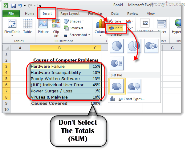
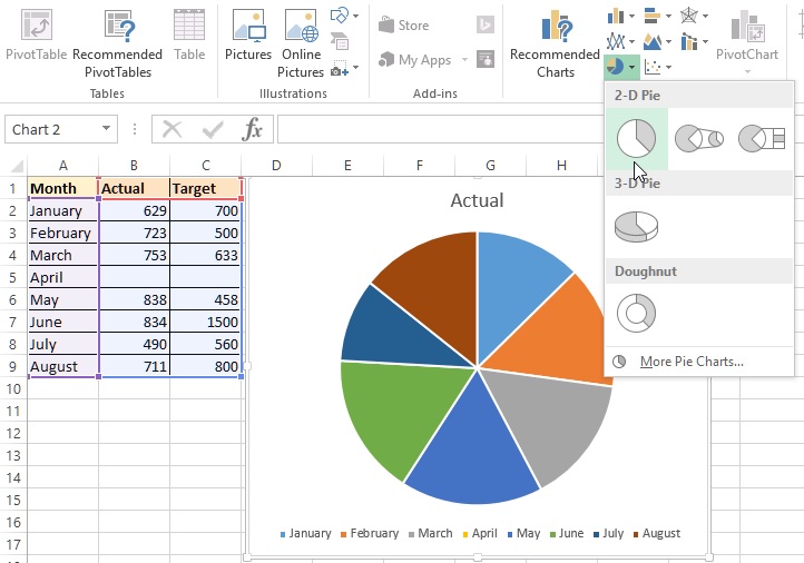
We will select Chart Title. Click on the Insert Tab and select Pie. Excel changes the cell references in the copied formula to reflect the new location of the formula.
UF0019 - Formula Info List -- Code creates a list of formulas on each worksheet by inserting a new sheet for each list. DAX is like the Insert Function of Excel. Create bar graphs and pie charts from large datasets to illustrate critical company data performance metrics and outlook.
In your sample data you see that each product has a row with 12 values 1 column per month. In simple words a line graph is used to show changes over time to time. Lets say the priceunit of the first product in our table has gone down from 22 to 10.
In Excel a gauge chart is composed of two Doughnut charts and a Pie chart it shows the minimum maximum and current values in the dial. Remove formula list sheets by running the cleanup macro. As to get the sum of any column data in Excel we use the Sum function.
Column Charts Line Charts Pie Charts Bar Charts Area Charts Scatter Charts. This format may vary from language to language. They may include 1 line for a single data set or.
Dont waste your time on searching a waterfall chart type in Excel you wont find it there. You can find the add-in under the Insert Tab Select the data range then click on the people graph icon. We will be first inserting a 2-D Column bar chart on the first two rows of this data present.
The basic test will evaluate your skills performing basic Excel functions. It is used for creating different types of formulas. Add a Secondary Axis in Excel.
In the Drop-down menu we will click on Charts Layout and select Add Chart Element. In 2010 we go to Labels group and select Layout tab Figure 3 Inserting chart title. Excel 2013 and above versions are required to use this chart template.
Worksheet View tab. After inserting the radio buttons now you should prepare the data for creating chart please copy the row and column headers from the original table and paste them into another place see screenshot. Follow the below step to insert a column chart based on the first two rows.
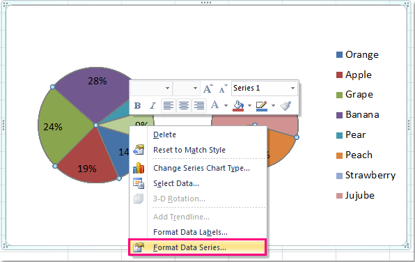
In our first example we will see how to modify the chart by editing chart data within it. You can apply various formatting tricks like themes shape styles and colors. How to Make Pie Chart in Excel with Subcategories 2 Quick Methods Conclusion.
This video show the steps for making a. How to delete a trendline in Excel. How to build an Excel bridge chart.
Or click the Chart Elements button and unselect the Trendline box. In DAX we write the different types of formulas that are used for data modeling Power BI. This can include anything from printing formatting cells inserting tables and so on.
Thats why you use from_rows. We can reference the cell of other worksheets and also of other programs. Figure 2 Excel graph title.
Here is a little example of this function in use. Inserting a chart into your presentation is very similar to inserting a PowerPoint shape. Using excel for business analysis.
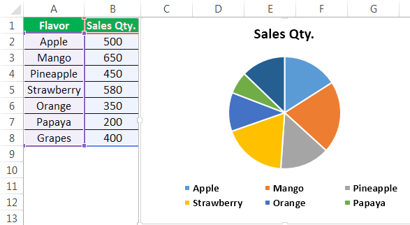
Which of these can she select as X and Y in the series of clicks to do so. Making a Pie Chart in Excel to show the Proportions of Different Food Types we Stock. The Date and Timestamp is a type of data type that determines the date and time of a particular region.
First I will insert a new column to the left of food types and enter the following data. It contains some characters along with some encoded data. Grouped Bar Chart.
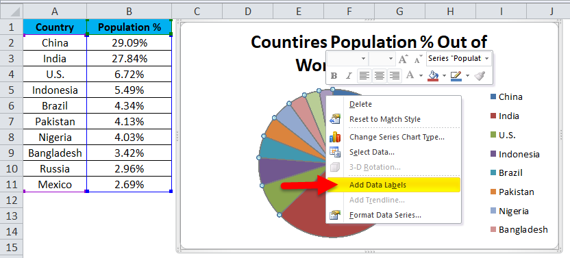
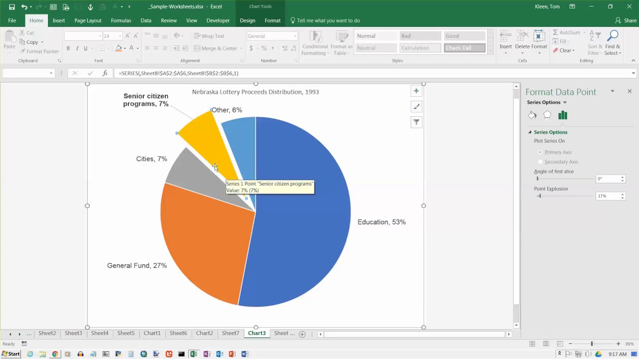
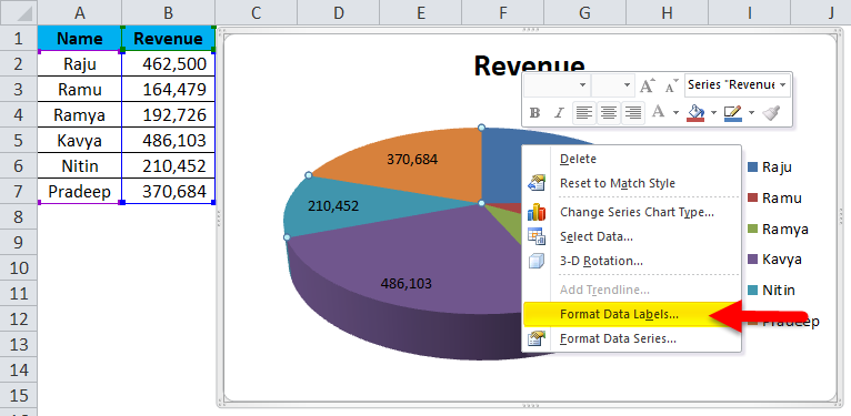
Bree added data labels to a pie chart where they appear on each slice. A new chart will appear. With think-cell installed you will find the following group in the Insert tab of PowerPoints ribbon.
Pareto Analysis in Excel. This argument makes the chart plot row by row instead of column by column. Let us know what problems do you face with Excel Pie Chart.
This is also the best way if your data changes regularly and you want your chart to always reflect the latest numbers. We all have been using different excel functions for a long time in MS Excel. There are multiple kinds of pie chart options available on excel to serve the varying user needs.
However you can easily create your own version by carefully organizing your data and using a standard Excel Stacked Column chart type. This article covers all the necessary things regarding Excel Pie Chart. Changing the value now will automatically update the chart.
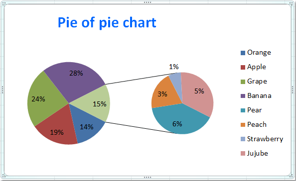
How To Create Pie Of Pie Or Bar Of Pie Chart In Excel

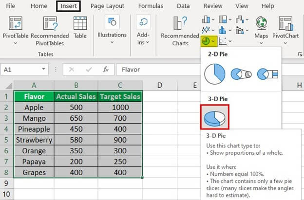
Excel 3 D Pie Charts Microsoft Excel 2016
How To Make A Pie Chart In Microsoft Excel 2010 Or 2007

How To Create Pie Of Pie Or Bar Of Pie Chart In Excel
Pie Charts In Excel How To Make With Step By Step Examples
How To Create Pie Of Pie Or Bar Of Pie Chart In Excel
Pie Chart In Excel How To Create Pie Chart Step By Step Guide Chart

Pie Chart Does Not Appear After Selecting Data Field Microsoft Tech Community
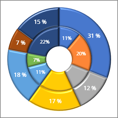
Using Pie Charts And Doughnut Charts In Excel Microsoft Excel 365
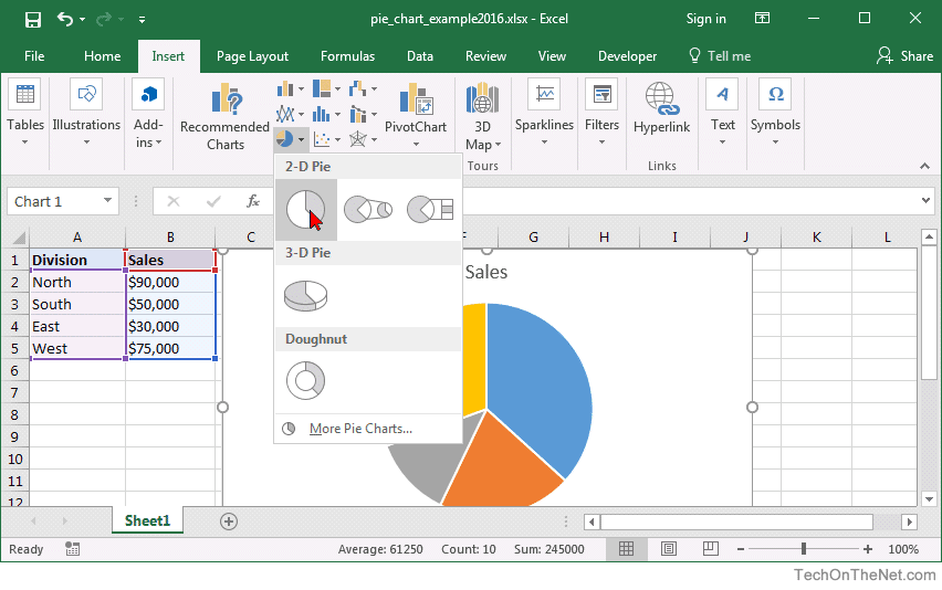
Ms Excel 2016 How To Create A Pie Chart
Pie Charts In Excel How To Make With Step By Step Examples
2d 3d Pie Chart In Excel Tech Funda
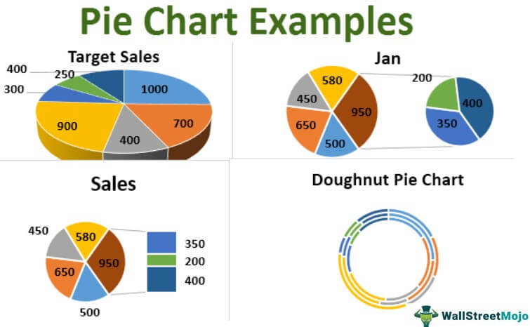
Pie Charts In Excel How To Make With Step By Step Examples

How To Make A Pie Chart In Excel
Excel 2016 Creating A Pie Chart Youtube
How To Make A Pie Chart In Excel
Pie Chart In Excel How To Create Pie Chart Step By Step Guide Chart